One of the most important topics in the field of machine learning is Gradient Descent which can be quite baffling at times. So, let us take a trip to understand the concept by getting our hands dirty with experiments and visualizations. I am going to use python programming language throughout the demonstrations.
First of all, what is Gradient Descent. Simply put, it is an algorithm working in the back-end of many regression model algorithms to fit a perfect fit line in a set of data points. We will be discussing everything in detail.
Let us take a classic example of the ‘Boston Housing Data Set’ for today’s discussion. The first few rows of data are presented below.
# Important imports
import warnings
warnings.filterwarnings('ignore')

import pandas as pd, numpy as np, matplotlib.pyplot as plt, seaborn as sns
from mpl_toolkits import mplot3d

from sklearn import datasets
from sklearn.linear_model import LinearRegression

from sklearn.metrics import mean_squared_error

# Loading dat
boston = datasets.load_boston()

# Creating dataframe
df = pd.DataFrame(boston['data'],columns=boston['feature_names'])
df['price'] = boston['target']

# Shuffling the dataframe
df = df.sample(n=len(df), random_state=20).reset_index(drop=True)

df.head()
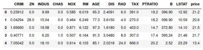
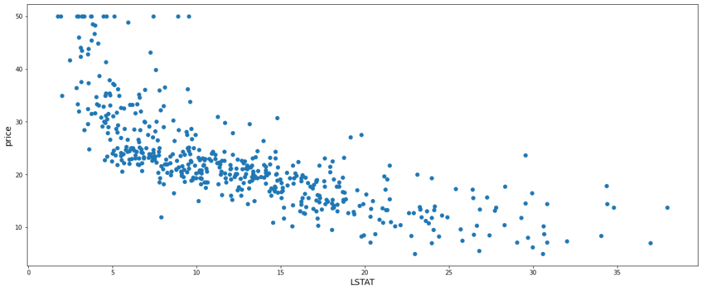
Let’s not dive deep into the meaning of each feature, rather let us just consider the existence of the above features as it is. ‘price’ column is the target variable that is to be predicted based on the other features. That is enough of the data introduction. For simplicity, let us consider one independent feature and the dependent variable itself for the demo. ‘LSTAT’ has been chosen among the independent variables since it has a good linear relationship with ‘price’ which will be visually efficient to understand. Hence, the scatter plot of our data, ‘LSTAT’ being in the x-axis and ‘price’ being in the y-axis is as follows:-
plt.figure(figsize=(20,8))
plt.scatter(df.LSTAT, df.price)
plt.xlabel('LSTAT', fontsize=14)
plt.ylabel('price', fontsize=14)
plt.show()
Now for prediction, we can perform Linear Regression. As the name suggests, linear regression refers to a process of fitting a linear instance of a curve, i.e., a straight line. The straight line is to be fit in such a way that the cost function is minimum or ideally 0.
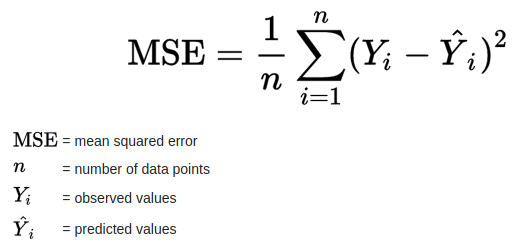
Here the cost function is Mean Squared Errors (MSE) which is nothing but the mean of all the squares of all vertical distances from each data point to the straight line. Mathematically, it can be summarized as follows :
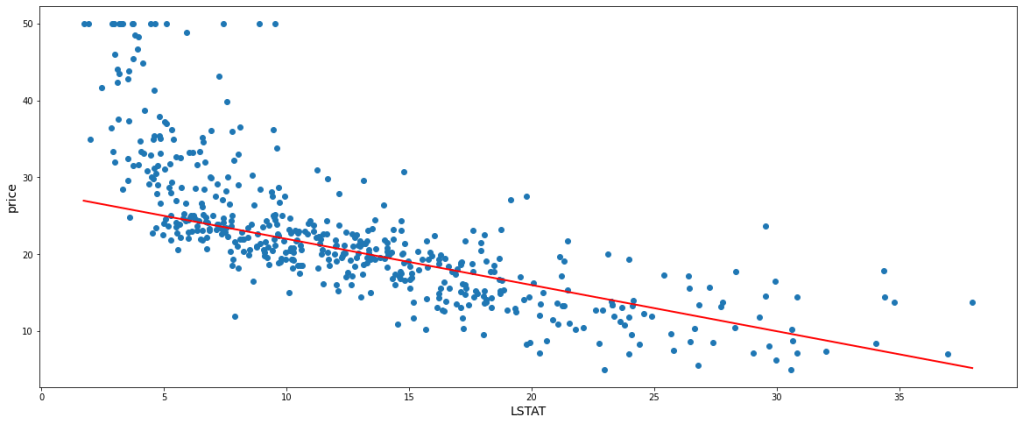
Now, the straight line that is to be fitted has a general equation y = mx + c where ‘m’ is the slope and ‘c’ is the intercept. These are the two parameters that structure and place the straight line. Let’s just fit a random line, say m = -0.2, c = 20, and get a glimpse.
# 'best_fit' is the custom function to fit the straight line with the provided coefficient and intercept
def best_fit(X,y,m,c):

    plt.figure(figsize=(20,8))

    # A scatter plot is produced for the data points
    plt.scatter(X, y)

    x = X.sort_values()
    # predictions are made based on the passed value of m and c
    predics = [(i*m)+c for i in x]

    # The predicted line is plotted in the same scatter plot graph
    plt.plot(x,predics, color='red', linewidth=2)
    plt.xlabel('LSTAT', fontsize=14)
    plt.ylabel('price', fontsize=14)
    plt.show()

############################################################################

best_fit(df.LSTAT,df.price,-0.2,20)
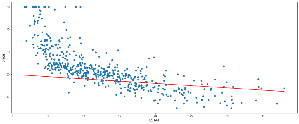
According to the above-fitted line, the predicted value of any value of x would be Ŷi = (-0.3 * xi) + 20 and the actual values (Yi) we already have. Therefore, we can easily calculate the value of the cost function which is equal to 92.75
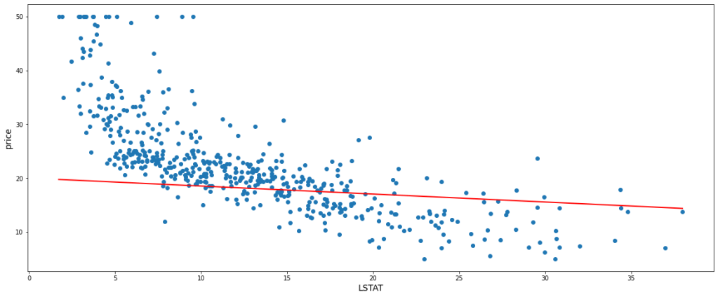
Let us take another instance with slight tweaking of m and c and fitting a new straight line at m = -0.6, c = 28. In this case, we get 49.23 as the cost function value. Below is the new model.
best_fit(df.LSTAT,df.price,-0.6,28)
This is evidently clear that if we can select a certain value of ‘m’ and ‘c’, we can attain a perfect fit straight line with a minimum cost function. But we can not choose values of m and c randomly, rather we need a systematic approach. For this purpose, the Gradient Descent algorithm comes into play.
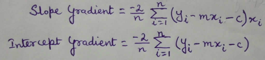
Let us get introduced to new terminology, Learning Rate. Here, it simply refers to a value that controls the change in slope and intercepts on the basis of cost function every time we build a new model. Slope and intercept gradients can be calculated by partial derivative of the cost function with respect to ‘m’ and ‘c’ respectively.
# 'gradients' function returns
def gradients(X,y,m,c):

    # Number of rows of data points
    N = len(X)

    # Prediction is done
    predicted = (m*X) + c

    # Gradients are calculated
    m_gradient = sum((y-predicted)*X)*(-2/N)
    c_gradient = sum(y-predicted)*(-2/N)
    return [m_gradient, c_gradient]


gradients(df.LSTAT,df.price,-0.2,20)
We have already seen a model previously at m = -0.2 and c = 20. Let the learning rate be = 0.001 On calculating the gradients with the above formulae, we get slope gradient = -51.79 and intercept gradient = -10.13 Now based on the learning rate and the gradients, the following set of formulae give the updated slope and intercept.
m = -0.2
c = 20
lrn = 0.001

# Slope gradient
m_gradient = gradients(df.LSTAT, df.price, m, c)[0]

# Intercept gradient
c_gradient = gradients(df.LSTAT, df.price, m, c)[1]

m = m - (lrn*m_gradient)
c = c - (lrn*c_gradient)
After updating the new slope, m = -0.14 and the new intercept, c = 20.01 With this new m and c, let’s fit a line within the data points and find the value of the cost function.
best_fit(df.LSTAT,df.price,m,c)
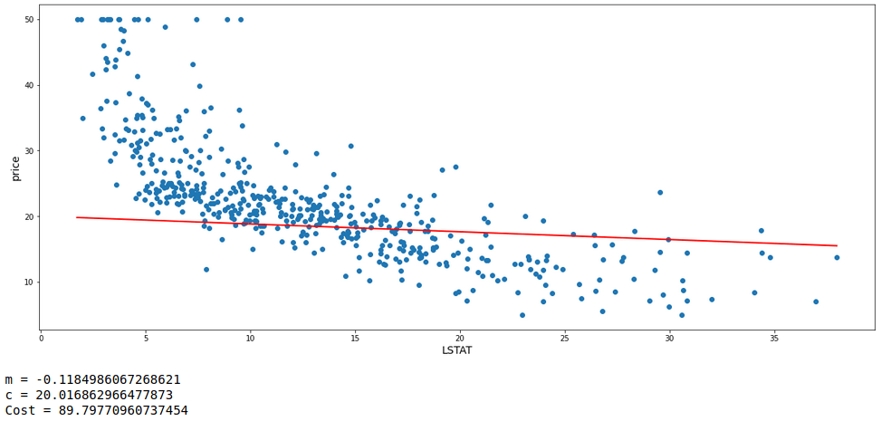
The model has a cost function value of 90.56 which is definitely less than the first model. Again we can update the values of m and c based on the values of learning rate and gradients and fit a new model which will hopefully give an improved fit with fewer errors. Thus we are going to see 2 more subsequent model fits each with a new updated value of m and c from its preceding model. We will also look at the values of m, c, and cost functions of each model.
m = m - (lrn*gradients(df.LSTAT, df.price, m, c)[0])
c = c - (lrn*gradients(df.LSTAT, df.price, m, c)[1])

best_fit(df.LSTAT,df.price,m,c)
print('m =',m)
print('c =',c)
print('Cost =',mean_squared_error(df.price, (m*df.LSTAT)+c))
m = m - (lrn*gradients(df.LSTAT, df.price, m, c)[0])
c = c - (lrn*gradients(df.LSTAT, df.price, m, c)[1])

best_fit(df.LSTAT,df.price,m,c)
print('m =',m)
print('c =',c)
print('Cost =',mean_squared_error(df.price, (m*df.LSTAT)+c))

It can clearly be seen that the errors are gradually decreasing. Thus after multiple iterations, it is probable to get a model with minimum error. It is like a ball freely rolling down a slope to reach the global minimum point of derivative of cost function.
In order to graphically establish the above-stated fact, a classic example image (Image Source) and animation (Animation Source) has been provided below for better understanding.
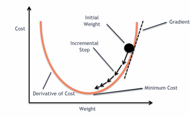
One fact to be kept in mind is that the learning rate can not be too large because in case it is too large, each leap will be large enough for the weight to ever reach the optimum level for the cost to be minimum. Let us see a demonstration of 3 consecutive models with m starting at -0.2, c at 20, and a high learning rate = 0.1 Along with each model, we will also have a look at the values of m, c, and cost.
lrn = 0.1
iters = 3

m=-0.2
c=20
m_gradient = gradients(df.LSTAT,df.price,m,c)[0]
c_gradient = gradients(df.LSTAT,df.price,m,c)[1]
print('\n\n')

i=1
while i<=iters:
    m = m-(lrn*m_gradient)
    c = c-(lrn*c_gradient)
    m_gradient = gradients(df.LSTAT,df.price,m,c)[0]
    c_gradient = gradients(df.LSTAT,df.price,m,c)[1]
    best_fit(df.LSTAT,df.price,m,c)
    print('m =',m)
    print('c =',c)
    print('Cost =',mean_squared_error(df.price, (m*df.LSTAT)+c))
    print('\n\n')
    i += 1
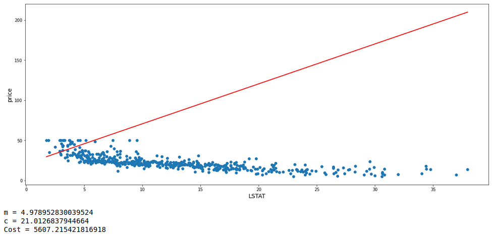
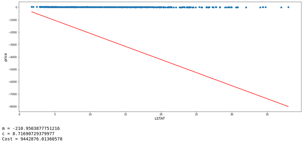
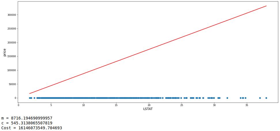
With the learning rate set high, it can be seen that the value of m is oscillating up and down instead of converging to the minimum cost value.
Now with all concepts and formulae set up, lets perform 20,000 iterations with m = 0, c = 0, learning rate = 0.001, and fit a straight line within the data points with the obtained value of m and c. Let’s have a look at the model fit and also the values of m, c, and cost of the model.
def gradient_descent(X, y, m_start=0, c_start=0, lrn=0.001, n_iter=10000):

    # A dataframe is initiated
    gradient_df = pd.DataFrame(columns=['m','c','cost'])

    # Value of m and c
    m = m_start
    c = c_start

    predicts = m*X + c
    cost = mean_squared_error(y,predicts)

    # 1st entry is made for the cost a initial values of m and c
    gradient_df.loc[0] = [m,c,cost]

    n = 1
    while n<=n_iter:
        m_grad = gradients(X,y,m,c)[0]
        c_grad = gradients(X,y,m,c)[1]

        m = m - m_grad*lrn
        c = c - c_grad*lrn

        predicts = m*X + c
        cost = mean_squared_error(y,predicts)

        gradient_df.loc[n] = [m,c,cost]

        n += 1

    return gradient_df


descent = gradient_descent(df.LSTAT,df.price,n_iter=20000)

req = descent[descent.cost==descent.cost.min()]
m = req.iloc[0,0]
c = req.iloc[0,1]
best_fit(df.LSTAT,df.price,m,c)

print('m =',m)
print('c =',c)
print('Cost =',mean_squared_error(df.price, (m*df.LSTAT)+c))
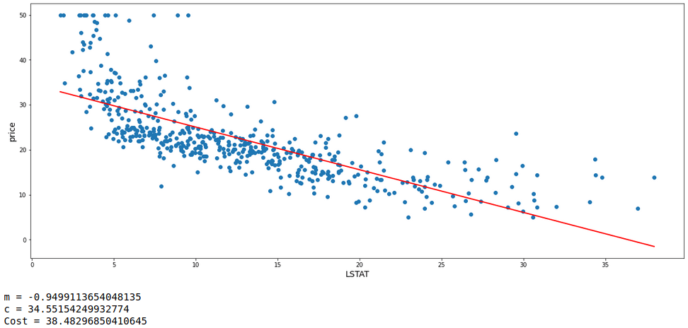
This is the best model achieved so far with the least error. In order to back this gradient descent performed, let’s automate this by building a Linear Regression model with ‘scikit-learn’ library in python to get the values of m, c, and cost.
# Linear Regression model is fit
model = LinearRegression().fit(X,y)

m = model.coef_[0]
c = model.intercept_

# 'best_fit' is the custom function to fit the straight line with the provided coefficient and intercept
best_fit(df.LSTAT,df.price,m,c)

print('m =',m,'\nc =',c,'\nCost =',mean_squared_error(df.price, (m*df.LSTAT)+c))

That was almost a wonderful match of the values between the model built manually and the one created by the automated process.
I hope I could successfully explain the basic concept of gradient descent algorithm. Now, it is time to move a step ahead. Let’s try to explore taking 2 features at a time. Therefore, I am choosing ‘LSTAT’ and ‘RM’ as the features along with ‘price’ as the target variable.
# 'multi' is the dataframe extract of the main data frame with one additional features
multi = df[['RM','LSTAT','price']]
multi.head()
This process follows the same principle and formulae as well. Only the difference is that sine there are multiple features involved, hence there will be multiple slopes for each feature. Thus for this, arrays are formed of slopes and used as matrices to perform calculations like multiplying each slope with its respective feature values during working out gradients, making predictions and many more.
# 'multi_gradient_descent' performs gradient descent over multiple features at a time
def multi_gradient_descent(X, y, m_start=0, c=0, lrn=0.001, n_iters=25000):

    store = pd.DataFrame(columns= [f'm_of_{i}' for i in X.columns] + ['c', 'cost'])

    ms = [{f'm{i}' : m_start} for i in X.columns]
    dic = {k:v for x in ms for k,v in x.items()}
    dic

    nos = 0
    while nos<=n_iters:

        res = []
        for i in range(len(X.columns)):
            mul = list(dic.values())[i] * X.iloc[:,i]
            res.append(mul)
        pred = sum(res) + c


        m_gradients = []
        for i in range(len(X.columns)):
            grad = (sum((y - pred)*X.iloc[:,i]) * (-2/len(X)))
            m_gradients.append(grad)

        m_gradients = np.array(m_gradients)


        c_gradient = sum(y - pred) * (-2/len(X))


        k=0
        for i in dic.keys():
            dic[i] = dic[i] - lrn*m_gradients[k]
            k += 1


        c = c - lrn*c_gradient


        res = []
        for i in range(len(X.columns)):
            mul = list(dic.values())[i] * X.iloc[:,i]
            res.append(mul)
        predicted = sum(res) + c


        cost = mean_squared_error(y,predicted)

        store.loc[nos] = list(dic.values())+[c,cost]


        nos += 1

    return store
X = multi.drop('price', axis=1)
y = multi.price

obt = multi_gradient_descent(X,y,n_iters=20000)

rr = obt[obt.cost == obt.cost.min()]

m = np.array(rr.iloc[0,:-2])
c = rr.c.values[0]
preds = np.matmul(X, m) + c

X = multi.drop('price', axis=1)
y = multi.price


# Creating dataset
a = np.array(X.LSTAT)
b = np.array(X.RM)
c = np.array(y)
p = preds

# Creating figure
plt.figure(figsize = (13,13))
ax = plt.axes(projection ="3d")

# Creating plot
ax.scatter3D(a, b, c, color = "green", s=8, label='actual')
ax.scatter3D(a, b, p, color = "red", s=8, label='predicted')

ax. set_xlabel('LSTAT', fontsize=13)
ax. set_ylabel('RM', fontsize=13)
ax. set_zlabel('price', fontsize=13)
plt.legend(fontsize=12)

ax.view_init(30,250)

# show plot
plt.show()


print('Cost =',mean_squared_error(y,preds))
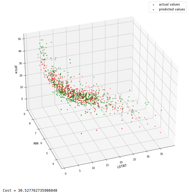
It seems there is a fairly nice match of patterns of actual and predicted values. Moreover, the cost value is lesser than the cost obtained in the model built with one feature only. For comparison purpose, let’s build a ‘scikit-learn’ Linear Regression model as well.
lr_multi = LinearRegression().fit(X,y)
lr_preds = lr_multi.predict(X)

# Creating dataset
a = np.array(X.LSTAT)
b = np.array(X.RM)
c = np.array(y)
p = lr_preds

# Creating figure
plt.figure(figsize = (13,13))
ax = plt.axes(projection ="3d")

# Creating plot
ax.scatter3D(a, b, c, color = "green", s=8, label='actual values')
ax.scatter3D(a, b, p, color = "magenta", s=8, label='predicted values')

ax. set_xlabel('LSTAT', fontsize=13)
ax. set_ylabel('RM', fontsize=13)
ax. set_zlabel('price', fontsize=13)
plt.legend(fontsize=12)

ax.view_init(30,250)

# show plot
plt.show()


print('Cost =',mean_squared_error(y,lr_preds))
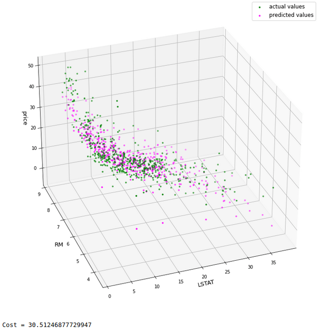
As we can see, there is a very good match between both the models with a comparable cost value.
Till now, we not only saw gradient descent but also saw that how does a Linear Regression works, that is, how it works behind the screen and attempts to do prediction.
