If you have gone through my Gradient Descent blog, you might have seen the demonstration of a model fits a line through the data points for prediction. The line that is fitted or preferably the model must be generalized. That simply means that the model must try to understand the basic trend rather than learning each and every data point by heart. Let’s try understanding with a demonstration. I would keep the demonstration as self-explainable as I can.
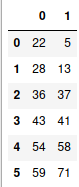
Alright, my current intention is to create an arbitrary dataframe so that I can produce an overfitting visualization. Let’s start by creating a very simple dataframe of 2 features and 6 rows of data points. Since topic is not regarding feature engineering, so I won’t be explaining this process of dataframe creation too much and rather would keep it short.
# Important imports
import warnings
warnings.filterwarnings('ignore')

import pandas as pd, numpy as np, matplotlib.pyplot as plt

from sklearn import datasets
from sklearn.linear_model import LinearRegression

from sklearn.metrics import mean_squared_error
from sklearn.preprocessing import MinMaxScaler, PolynomialFeatures


base = pd.DataFrame({'0':[22,28,36,43,54,59],
                  '1':[5,13,37,41,58,71]})
base
Now let’s transform the independent variable to 5th degree polynomial.
scaler = MinMaxScaler()
base[base.columns] = scaler.fit_transform(base[base.columns])

X = base.iloc[:,0]
y = base.iloc[:,1]

df = pd.DataFrame(PolynomialFeatures(5).fit_transform(sorted(X.values.reshape(-1,1))))
df['label'] = y
df
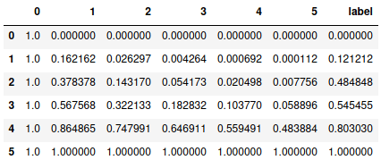
Now we have got a dataframe with 6 features and a label. Now using the same process and function as used in the Gradient Descent blog, let’s perform gradient descent for multiple features and fit a best fit line or curve. Then plot the predictions and actual values with respect to feature in the ‘base’ dataframe and look at the cost value.
def multi_gradient_descent(X, y, m_start=0, c=0, lrn=0.001, n_iters=25000):
store = pd.DataFrame(columns= [f'm_of_{i}' for i in X.columns] + ['c', 'cost'])
# m0=m1=m2=m3=m4=m5 = m_start
ms = [{f'm{i}' : m_start} for i in X.columns]
dic = {k:v for x in ms for k,v in x.items()}
dic
nos = 0
while nos<=n_iters:
res = []
for i in range(len(X.columns)):
mul = list(dic.values())[i] * X.iloc[:,i]
res.append(mul)
pred = sum(res) + c
m_gradients = []
for i in range(len(X.columns)):
grad = (sum((y - pred)*X.iloc[:,i]) * (-2/len(X)))
m_gradients.append(grad)
m_gradients = np.array(m_gradients)
c_gradient = sum(y - pred) * (-2/len(X))
k=0
for i in dic.keys():
dic[i] = dic[i] - lrn*m_gradients[k]
k += 1
c = c - lrn*c_gradient
res = []
for i in range(len(X.columns)):
mul = list(dic.values())[i] * X.iloc[:,i]
res.append(mul)
predicted = sum(res) + c
cost = mean_squared_error(y,predicted)
store.loc[nos] = list(dic.values())+[c,cost]
nos += 1
return store
X = df.drop('label', axis=1)
y = df.label
obt = multi_gradient_descent(X,y,lrn=0.1,n_iters=20000)
min_cost = obt[obt.cost == obt.cost.min()]
m_overfit = np.array(min_cost.iloc[0,:-2])
c_overfit = min_cost.c.values[0]
preds_overfit = np.matmul(X, m_overfit) + c_overfit
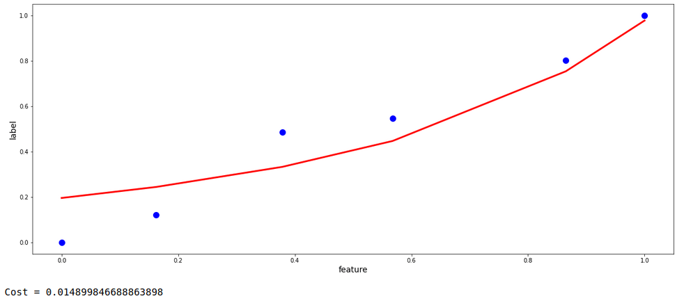
plt.figure(figsize=(20,8))
plt.scatter(base.iloc[:,0], y, s=100, c='blue')
plt.plot(base.iloc[:,0], preds_overfit, color='red', linewidth=3)
plt.xlabel('feature', fontsize=14)
plt.ylabel('label', fontsize=14)
plt.show()
print('Cost =',mean_squared_error(y,preds_overfit))
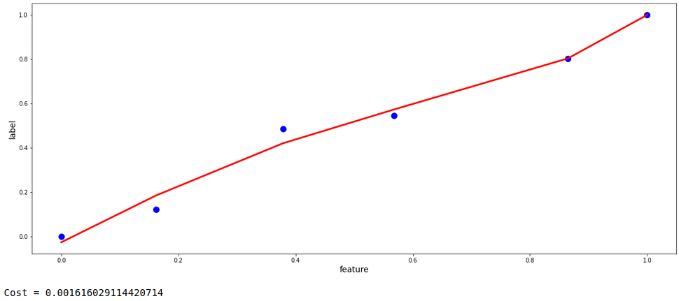
Looking at the model above, it is evident that the model is moderately overfitting. The model is not generalized, rather is trying to learn all the provided data points as it is by compromising the errors and learning the noise in the data set as well . If we extend the graph using the same coefficients as obtained during the process of gradient descent, it can be imagined that the predictions would not be fair and could have bias for future data.
To resolve this problem, Regularization is performed. Two of the most common process of regularization are Ridge and Lasso Regression.
Regularization
The approach is simple : we add a term to the cost function.
Ridge Regression Cost = MSE(m) + λ*||m||²
where m is the slope, λ is a constant. Mean squared error is calculated at m and the term λ*||m||² is added to it.
The gradients are found by differentiating this entire cost function itself and during each iteration, slopes and intercepts are updated using these gradients.
Therefore, the gradients for this are as follows:-
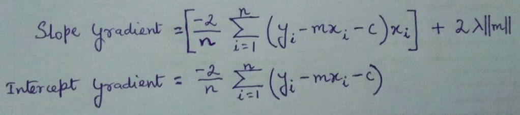
From the equations it is clear that slop gradient is directly proportional to λ. Therefore as λ increases, updated slope decreases given that learning rate is constant. More the value of λ, rapid the decrease of slope will occur. The slopes will consequently tend towards 0 but will never actually 0. This is mathematically represented below.
updated_m = learning rate * slope gradient For updated_m to be 0 in Ridge Regression, the following has to me true: m = learning rate * slope gradient => m = a + ( b * ||m|| ) where,Since m ≠ a + ( b * ||m|| ) due to the presence of ||m|| on the RHS, Therefore, updated_m cannot be 0.
In the other type of regularization, i.e., Lasso Regression, λ*||m|| is added to the regular cost function instead of λ*||m||² . This brings some changes like in the slope gradient, the last term will be only λ instead of 2*λ*||m||. This will eventually cause many slopes of certain features turn to 0, which is explained below.
updated_m  =  learning rate * slope gradient
For updated_m to be 0 in Lasso Regression, the following has to me true:
   m  =  learning rate * slope gradient
=> m  =  a + b

where a is same as before whereas,
b = learning rate * λ

Therefore for Lasso Regression, updated_m can absolutely be 0.
For today’s topic, let’s use Ridge Regression for regularization. Below is give the function for multiple gradient descent with the corresponding cost function. If you notice carefully, the gradient equation has also be changed accordingly.
def multi_regular_gradient_descent(X, y, lamda=0.01, m_start=0, c=0, lrn=0.001, n_iters=25000):

    store = pd.DataFrame(columns= [f'm_of_{i}' for i in X.columns] + ['c', 'cost'])


    ms = [{f'm{i}' : m_start} for i in X.columns]
    dic = {k:v for x in ms for k,v in x.items()}
    dic

    nos = 0
    while nos<=n_iters:

        res = []
        for i in range(len(X.columns)):
            mul = list(dic.values())[i] * X.iloc[:,i]
            res.append(mul)
        pred = sum(res) + c


        m_gradients = []
        for i in range(len(X.columns)):
            abs_slopes = [abs(i) for i in list(dic.values())]
            grad = (sum((y - pred)*X.iloc[:,i]) * (-2/len(X))) + (2*lamda*abs_slopes[i])
            m_gradients.append(grad)

        m_gradients = np.array(m_gradients)


        c_gradient = sum(y - pred) * (-2/len(X))


        k=0
        for i in dic.keys():
            dic[i] = dic[i] - lrn*m_gradients[k]
            k += 1


        c = c - lrn*c_gradient

        res = []
        for i in range(len(X.columns)):
            mul = list(dic.values())[i] * X.iloc[:,i]
            res.append(mul)
        predicted = sum(res) + c


        cost = mean_squared_error(y,predicted)

        store.loc[nos] = list(dic.values())+[c,cost]


        nos += 1


    return store
As the function has been defined, let’s perform gradient descent in the same dataset. If you have already gone through my Gradient Descent blog, you will be familiar with almost all the parameters. Parameters: λ = 0.1, learning rate = 0.1, number of iterations = 20,000, m and c both starting with 0.
X = df.drop('label', axis=1)
y = df.label

obt = multi_regular_gradient_descent(X,y,lamda=0.1,lrn=0.1,n_iters=20000)

min_cost = obt[obt.cost == obt.cost.min()]

m_regular = np.array(min_cost.iloc[0,:-2])
c_regular = min_cost.c.values[0]

preds_regular = np.matmul(X, m_regular) + c_regular


plt.figure(figsize=(20,8))
plt.scatter(base.iloc[:,0], y, s=100, c='blue')
plt.plot(base.iloc[:,0], preds_regular, color='red', linewidth=3)
plt.xlabel('feature', fontsize=14)
plt.ylabel('label', fontsize=14)
plt.show()

print('Cost =',mean_squared_error(y,preds_regular))
Now, this model’s fit is pretty much generalized without any aggressive tendency to fit to the data points. Let’s do the same with the automated process provided by the ‘scikit-learn’ library in python and compare them both with respect to fit and the cost value.
lr = Ridge(alpha=0.1).fit(X,y)
preds_lr = lr.predict(X)

plt.figure(figsize=(20,8))
plt.scatter(base.iloc[:,0], y, s=100, c='blue')
plt.plot(base.iloc[:,0], preds_lr, color='red', linewidth=3)
plt.xlabel('age', fontsize=14)
plt.ylabel('salary', fontsize=14)
plt.show()

print('Cost =',mean_squared_error(y,preds_lr))
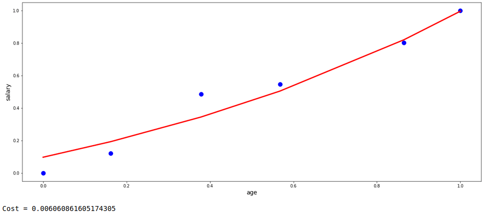
Even if both are not precisely the same, but still we got a fairy good degree of regularization with almost similar cost value and curve fit structure.
Remember, it is always recommended to use the trusted tools and libraries available to build models instead of any scratch coded functions like the one I presented. These scratch codes are just for showing an overview of the back-end processes.
I hope I could explain the concepts. For any suggestion, feel free to contact me.
