This is a pretty short and simple way to verify our hypothesis. This test simply suggests whether a given categorical feature in a dataframe is significant for prediction of the dependent variable or not. We will move straight towards performing a simple test.
Let us consider the null hypothesis to be that a given feature is insignificant whereas the alternate hypothesis to be that the feature is significant enough.
As usual, first of all let’s build an arbitrary dataframe for our purpose.
dic = {'very_short': [12,  3, 15],
       'short': [16,  9, 25],
       'moderate': [ 2, 13, 15],
       'long': [ 5, 35, 40],
       'very_long': [12,  7, 19],
       'total': [ 47,  67, 114]}

obs = pd.DataFrame(dic).rename(index={2:'total'})
obs
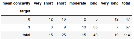
Note: This dataframe is created as the form of replica when crosstab fuction is applied on any pandas dataframe. You can read about crosstab here.
Here, we are going to find the significance of the feature length (very short, short, moderate, long, very long) with respect to the binary class (1 and 0). Otherwise, the information in the dataframe is self-explainable. All the values here are called the observed values. With respect to this, we need to calculate the expected values. The way to calculate the expected values is as follows:
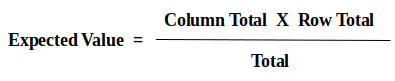
For eg., at (0,0) value will be = (47*15)/114 ; at (1,3) value will be = (67*40)/114
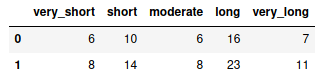
Therefore, the expected values are as follows:
arr = np.array(obs)

rows = arr[:-1,:-1].shape[0]
cols = arr[:-1,:-1].shape[1]


for row in range(0,rows):
    for col in range(0,cols):
        arr[row,col] = ((arr[row,5]*arr[2,col])/arr[rows,cols])

arr = arr[:-1,:-1]

exp = pd.DataFrame(arr, columns=obs.columns[:-1], index=obs.index[:-1])
exp
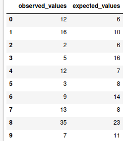
Now all the corresponding observed and expected values are listed.
obs_vals = [obs.loc[row,col] for row in obs.iloc[:-1,:-1].index for col in obs.iloc[:-1,:-1].columns]
exp_vals = [exp.loc[row,col] for row in exp.index for col in exp.columns]
chi = pd.DataFrame({'observed_values':obs_vals, 'expected_values':exp_vals})
chi
There are some other subsequent calculations are involved as well which could be self explained through the following table:
chi['observed_values - expected_values'] = chi.observed_values - chi.expected_values
chi['square(observed_values - expected_values)'] = chi['observed_values - expected_values']**2
chi['square(observed_values - expected_values)/expected_values'] = chi['square(observed_values - expected_values)'] / chi.expected_values
chi

chi_square = chi['square(observed-expected)/expected'].sum()
chi_square
The summation of the last column, i.e., ‘the square of difference of observed and expected values divided by the expected values’ gives us the value of the calculated chi-square (χ2) which comes out to be 39.15
Now, it is time to work out the degree of freedom. Degree of freedom (DOF) is given by the following expression:
DOF = (No. of rows – 1) * (No. of columns – 1)
dof = (rows-1)*(cols-1)
dof
Using the above code we can find the degree of freedom to be 4. Now, we can find the critical value of chi-square from the Chi-Squared distribution table, provided below based on the calculated degree of freedom:
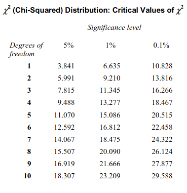
From the above table, we can see that for degree of freedom 4 and 0.1% significance level, critical value of chi-squared is 18.467.
Since, therefore, the mentioned feature is significant for prediction.
Thus, we can reject the null hypothesis and accept the alternate hypothesis.
Had the condition been vice versa, i.e., calculated chi-squared is less than the critical chi-squares, then we would have failed to reject the null hypothesis.
