In simple words, clusters are groups of data points in the space within which the data points have similar characteristics. Whereas, data points from different clusters have significantly different characteristics. Let’s straight away visualize such a scenario.
def making_df(n=100, p1=100, p2=30, p3=2):
    np.random.seed(n)

    p=np.random.randn(p1)*p2
    q=np.random.randn(p1)*p2

    w=p
    x=q-2*p3*q.max()


    r=p+p3*p.max()
    s=q-p3*q.max()


    df0 = pd.DataFrame({'feature1':w,
                       'feature2':x, 'label':[0]*len(r)})
    df1 = pd.DataFrame({'feature1':p,
                       'feature2':q, 'label':np.ones(len(p))})

    df2 = pd.DataFrame({'feature1':r,
                       'feature2':s, 'label':[-1]*len(r)})

    df = pd.concat([df0,df1,df2], axis=0)
    df = df.sample(n=len(df))
    df = df.reset_index(drop=True)
    return [df,p,q,r,s,w,x]
This function helps in creating an arbitrary dataframe of our choice. Let’s build one for understanding purpose.
df,p,q,r,s,w,x = making_df()

plt.figure(figsize=(20,8))
plt.scatter(df.feature1,df.feature2)
plt.show()
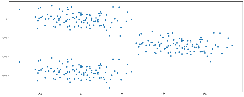
Looking at the plot, we can say that there are fairly 3 clusters present in the data set.
Clustering is a kind of unsupervised learning algorithm, i.e., we are not provided with labels rather we do segmentation based on their features. For our sake of understanding, let’s consider K-Means clustering for the topic and see how the algorithm works.
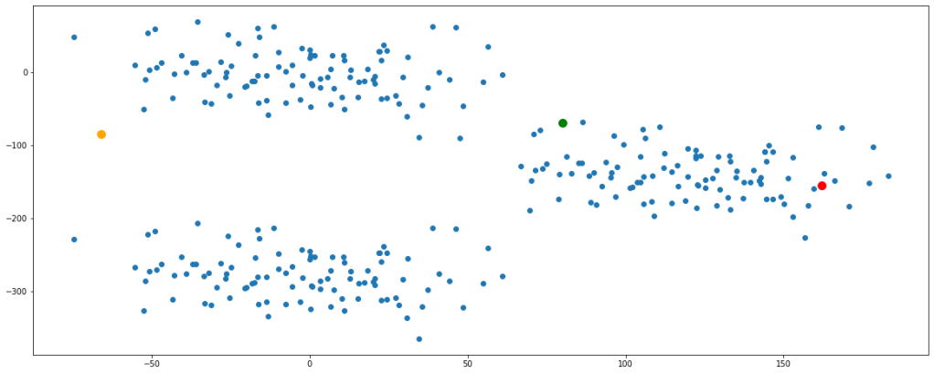
Step 1:
Initiate cluster centers, also calledcentroids at random in the space. Let us take 3 cluster centers and randomly fit them in the space.
seeds = [55,100,8000]

np.random.seed(seeds[0])
a = np.random.randint(df.feature1.min(),df.feature1.max())
b = np.random.randint(df.feature2.min(),df.feature2.max())

np.random.seed(seeds[1])
c = np.random.randint(df.feature1.min(),df.feature1.max())
d = np.random.randint(df.feature2.min(),df.feature2.max())

np.random.seed(seeds[2])
e = np.random.randint(df.feature1.min(),df.feature1.max())
f = np.random.randint(df.feature2.min(),df.feature2.max())

plt.figure(figsize=(20,8))
plt.scatter(df.feature1,df.feature2)
plt.scatter(a,b, color='green', s=100)
plt.scatter(c,d, color='orange', s=100)
plt.scatter(e,f, color='red', s=100)
plt.show()
Before proceeding ahead, let’s get clarified about Euclidean distance since this term will be used extensively. Wherever I say distance, I would actually mean ‘Euclidean Distance’. Euclidean distance is nothing but the formulation of the length of the hypotenuse in a right-angled triangle. You can read more about this by clicking here.
After the initialization of centroids, we calculate the distance of each point from each of the centroids.
def euc(x1,x2,y1,y2):
    dist = ((x1-x2)**2 + (y1-y2)**2)**0.5
    return dist

for i in range(5):
    cluster1 = euc(a,df.feature1,b,df.feature2)
    cluster2 = euc(c,df.feature1,d,df.feature2)
    cluster3 = euc(e,df.feature1,f,df.feature2)

    cluster = pd.concat([cluster1,cluster2,cluster3], axis=1)
    cluster.columns=['cluster1','cluster2','cluster3']


cluster
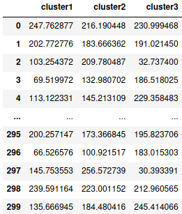
This dataframe gives us the distance of each data point represented by their index numbers with each centroid of their respective clusters. The thumb rule is that a data point will be considered to the cluster with the centroid of which it has the shortest distance.
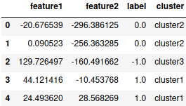
Depending on these distances let’s classify the data points in either of the 3 clusters.
dic = {}
for i in cluster.index:
    dic[i]=cluster.columns[np.argmin(cluster.iloc[i])]

df['cluster'] = dic.values()

df.head()
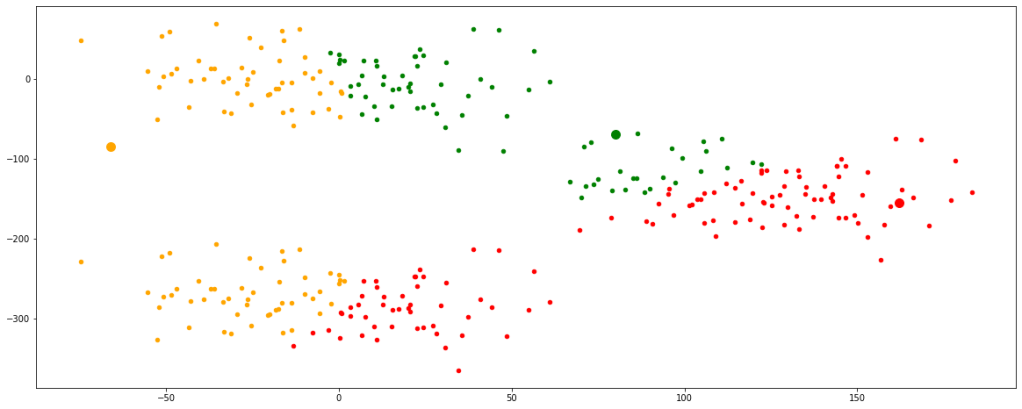
Let’s visualize the clusters formed with these newly initialized centroids.
plt.figure(figsize=(20,8))
plt.scatter(a,b, color='green', s=100)
plt.scatter(c,d, color='orange', s=100)
plt.scatter(e,f, color='red', s=100)

new = df[df.cluster=='cluster1']
plt.scatter(new.feature1,new.feature2, color='green', s=20)

new = df[df.cluster=='cluster2']
plt.scatter(new.feature1,new.feature2, color='orange', s=20)

new = df[df.cluster=='cluster3']
plt.scatter(new.feature1,new.feature2, color='red', s=20)

plt.show()

Step 2:
As we can see the clusters formed are not optimum, therefor we must update the centroids. It is done by taking the mean of the coordinates of data points in their respective clusters.
new = df[df.cluster=='cluster1']
a=new.feature1.mean()
b=new.feature2.mean()

new = df[df.cluster=='cluster2']
c=new.feature1.mean()
d=new.feature2.mean()

new = df[df.cluster=='cluster3']
e=new.feature1.mean()
f=new.feature2.mean()
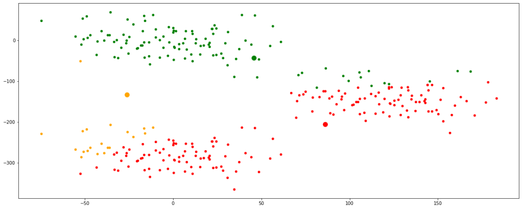
Step 3:
The updated centroids are assigned again in the data space, distances from each data point are calculated and corresponding clusters are formed.
def euc(x1,x2,y1,y2):
    dist = ((x1-x2)**2 + (y1-y2)**2)**0.5
    return dist

for i in range(5):
    cluster1 = euc(a,df.feature1,b,df.feature2)
    cluster2 = euc(c,df.feature1,d,df.feature2)
    cluster3 = euc(e,df.feature1,f,df.feature2)

    cluster = pd.concat([cluster1,cluster2,cluster3], axis=1)
    cluster.columns=['cluster1','cluster2','cluster3']


dic = {}
for i in cluster.index:
    dic[i]=cluster.columns[np.argmin(cluster.iloc[i])]

df['cluster'] = dic.values()


plt.figure(figsize=(20,8))
plt.scatter(a,b, color='green', s=100)
plt.scatter(c,d, color='orange', s=100)
plt.scatter(e,f, color='red', s=100)

new = df[df.cluster=='cluster1']
plt.scatter(new.feature1,new.feature2, color='green', s=20)

new = df[df.cluster=='cluster2']
plt.scatter(new.feature1,new.feature2, color='orange', s=20)

new = df[df.cluster=='cluster3']
plt.scatter(new.feature1,new.feature2, color='red', s=20)

plt.show()

Now, we can see that the centroids have moved a bit and are tending towards their respective clusters. After multiple iterations, we will find the centroids not changing any further and thus we would have finally achieved the final set of clusters.
Let’s look at multiple iterations by accumulating all the above codes in a single function for our ease of execution. We would see every change occurring in the position of the centroids.
def clust(seeds):

    np.random.seed(seeds[0])
    a = np.random.randint(df.feature1.min(),df.feature1.max())
    b = np.random.randint(df.feature2.min(),df.feature2.max())

    np.random.seed(seeds[1])
    c = np.random.randint(df.feature1.min(),df.feature1.max())
    d = np.random.randint(df.feature2.min(),df.feature2.max())

    np.random.seed(seeds[2])
    e = np.random.randint(df.feature1.min(),df.feature1.max())
    f = np.random.randint(df.feature2.min(),df.feature2.max())

    plt.figure(figsize=(20,8))
    plt.scatter(df.feature1,df.feature2)
    plt.scatter(a,b, color='green', s=100)
    plt.scatter(c,d, color='orange', s=100)
    plt.scatter(e,f, color='red', s=100)
    plt.show()


    def euc(x1,x2,y1,y2):
        dist = ((x1-x2)**2 + (y1-y2)**2)**0.5
        return dist


    for i in range(5):
        cluster1 = euc(a,df.feature1,b,df.feature2)
        cluster2 = euc(c,df.feature1,d,df.feature2)
        cluster3 = euc(e,df.feature1,f,df.feature2)


        cluster = pd.concat([cluster1,cluster2,cluster3], axis=1)
        cluster.columns=['cluster1','cluster2','cluster3']


        dic = {}
        for i in cluster.index:
            dic[i]=cluster.columns[np.argmin(cluster.iloc[i])]

        df['cluster'] = dic.values()


        plt.figure(figsize=(20,8))
        plt.scatter(a,b, color='green', s=100)
        plt.scatter(c,d, color='orange', s=100)
        plt.scatter(e,f, color='red', s=100)


        new = df[df.cluster=='cluster1']
        plt.scatter(new.feature1,new.feature2, color='green', s=20)
        a=new.feature1.mean()
        b=new.feature2.mean()

        new = df[df.cluster=='cluster2']
        plt.scatter(new.feature1,new.feature2, color='orange', s=20)
        c=new.feature1.mean()
        d=new.feature2.mean()

        new = df[df.cluster=='cluster3']
        plt.scatter(new.feature1,new.feature2, color='red', s=20)
        e=new.feature1.mean()
        f=new.feature2.mean()

        plt.show()
clust([55,100,8000])

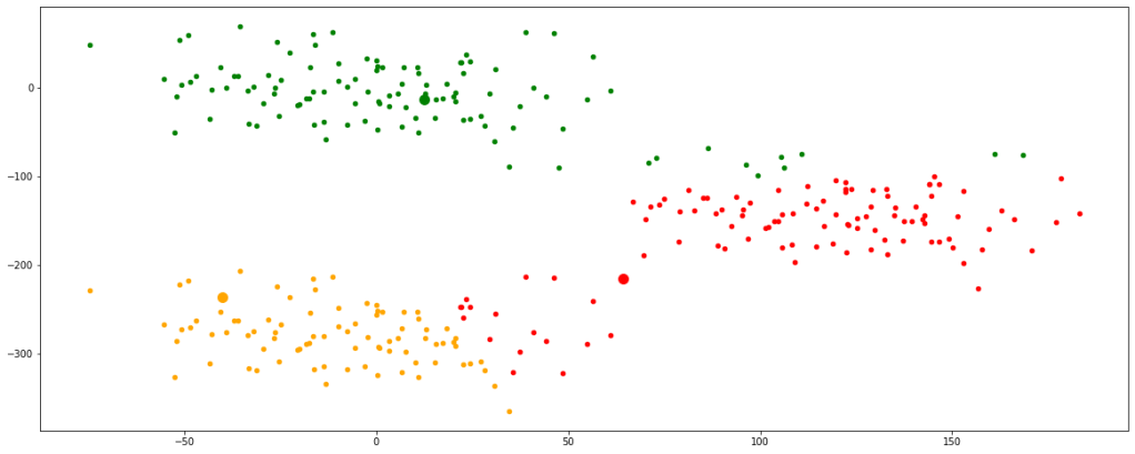
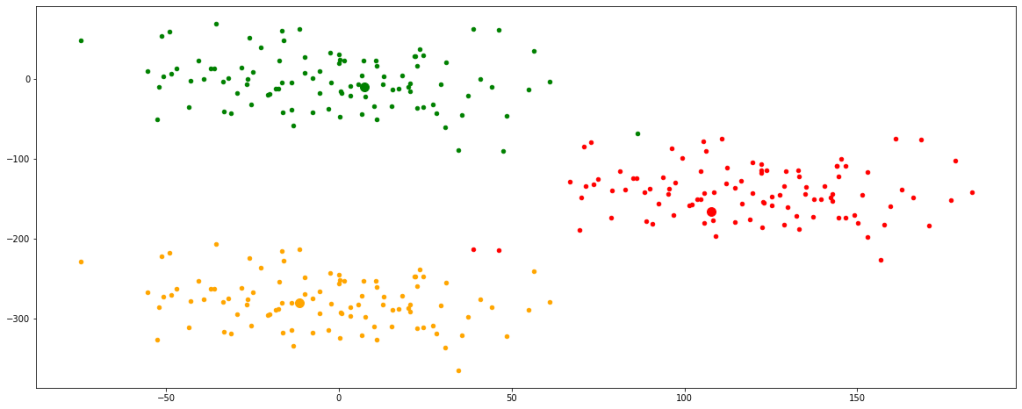
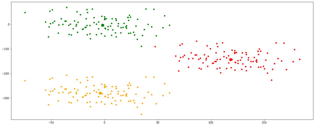
Now, we have finally obtained 3 valid clusters after 6 iterations. Analogically similar processes would be followed in higher dimension data sets as well.
K-Means clustering can be performed using the ‘sklearn’ library in python. You can read more about this by clicking here.
This kind of clustering has some drawbacks as well. Some of them being they are only valid for numeric data types. They cannot handle categorical data types. Moreover, K-Means do not perform well with outliers since if there is any, the updation of centroids would be highly affected and will get skewed towards the outlier. It does not perform well even with data sets with varying data densities.
