PCA

PCA stands for Principal Component Analysis. To explain in simple words, it is a process of dimensional reduction of data without loosing any significant information. We will be looking towards the entire algorithm and understand step by step. Let’s first build an arbitrary data set and plot it to have a visual representation of the data we will be dealing with.

import pandas as pd, numpy as np, matplotlib.pyplot as plt, seaborn as sns

np.random.seed(100)
x = np.random.sample(10)
y = 0.4*x + 2
df = pd.DataFrame({'x':x,'y':y})

df

plt.figure(figsize=(20,8))
plt.scatter(df.x,df.y)
plt.xlabel('x', fontsize=16)
plt.ylabel('y', fontsize=16)
plt.show()

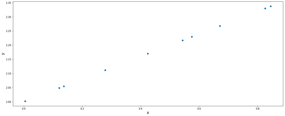
From this data set, we can say that in order to represent these set of data, we need 2 dimensions. But what if we could use only 1 dimension instead of 2? This is what PCA helps us with. The dimensionality reduction helps us in various ways:

• In case of many dimensions, we can reduce the dimensions so that we can visually represent the data.
• Processing less dimension data aids in computational efficiency.

Simple explanation is that he PCA performs this task by rotating the Cartesian coordinates such that one coordinate lies on the data points (with maximum variance or information).

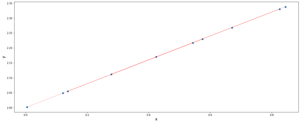
We can imagine the red line to be the x-axis which got transformed in such a way that now it lies over the data points. If that could be the case and we could find such transformations, dimensionality reduction would surely be possible.

In order to understand the algorithm, we must be familiar with certain terms:

• Covariance matrix – It is a symmetric, positive and a square matrix with the covariance between each pair of elements of a given random vector. Covariance is a big topic in itself. You may click here for reading more about covariance.
• Eigenvectors – The vectors formed after transforming another vector which does not change direction rather gets scaled at most are called eigenvectors.
• Eigenvalues – The scaler value by which a vector gets scaled after transformation, corresponding to the eigenvector is applied is called eigenvalue.
• Basis – The current basis is [[0,1],[1,0]]. These are the coordinates of the current x and y axis which are also called basis. Our aim is to find a new basis which satisfies our need of transformation.

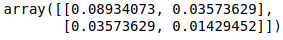
Let’s find the covariance matrix for the dataframe first.

cov = np.cov(np.array(df).T)
cov

Now, let’s find the eigenvectors corresponding to the above covariance.

eig = np.linalg.eig(cov)
eig_vectors = eig[1]
eig_vectors

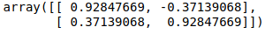
Now, this is our new basis. Let’s perform a dot product to the data points with this new basis.

new = df @ eig_vectors
new.columns = ['Principal Component 1','Principal Component 2']
new

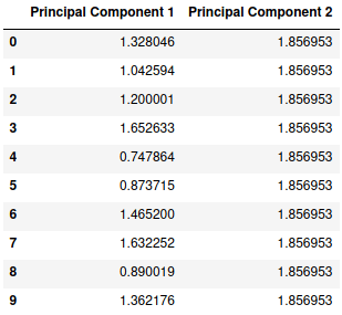
We can clearly see that principal component 1 itself has all the information and variance stored whereas the principal component 2 has a constant value of 1.856953 which provides us with no useful information. Let’s plot this new set of data.

plt.figure(figsize=(20,8))
plt.scatter(new['Principal Component 1'],new['Principal Component 2'])
plt.axhline(y=new['Principal Component 2'][0], linewidth=0.5, color='red')
plt.xlabel('x', fontsize=16)
plt.ylabel('y', fontsize=16)
plt.show()

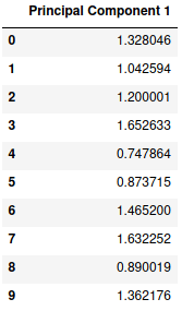
Thus, we have successfully obtained our desired transformation. We can see that the data points are defined by a single dimension itself and therefore we can ignore the second principal component and our final data set will look like this:

new = new.drop('Principal Component 2', axis=1)
new

Analogically, we can imagine the working of PCA in higher dimensions as well.

—END—